Volatility Models: GARCH, Realized Volatility, HAR
When does a GARCH forecast differ materially from realized-volatility alternatives?
Fit competing forecasts only on information available before each prediction, then compare their held-out volatility errors under the same horizon and loss function. A realized-volatility measure based on 78 five-minute intervals describes a US cash session, not a full FX day.
The 78 five-minute intervals describe a US cash-equity session, not a full FX day.
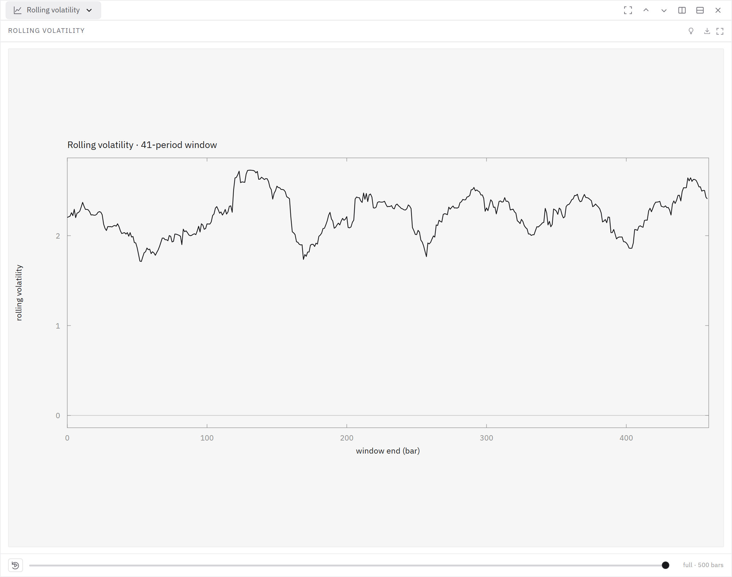
Evidence map
| Aspect | Finding |
|---|---|
| What it is | The two families used to forecast conditional variance. GARCH models variance recursively from past returns; realized volatility estimates it directly by summing intraday squared returns, and HAR forecasts that realized measure with a cascade of horizons. |
| Key result / formula | GARCH(1,1): σ²_t = ω + α·ε²_{t-1} + β·σ²_{t-1}, stationary when α + β < 1, with α + β typically close to one on daily equity data — the persistence that makes volatility forecastable at all. |
| Why it matters for backtesting | Volatility is the one quantity in finance that is genuinely predictable, and each risk control depends on that forecast: position sizing, volatility targeting, stop placement, drawdown limits. |
Key result / formula
Realized variance: RV_t = Σ_i r²_{t,i} over intraday intervals, a consistent estimator of integrated variance as the sampling interval shrinks, but contaminated by microstructure noise at very high frequency (hence the standard compromise of five-minute sampling, or noise-robust estimators). Corsi's HAR model regresses RV on its own daily, weekly and monthly averages — a simple linear specification that reproduces long-memory behaviour and is hard to beat out of sample.
Why it matters for backtesting
Two warnings. Forecasting variance well implies no skill at forecasting direction — these models are sign-blind by construction, and a good volatility model is routinely mistaken for evidence of a directional edge. And the asymmetry matters: negative returns raise future volatility more than positive ones (the leverage effect, captured by GJR-GARCH or EGARCH), so a symmetric model underestimates risk exactly after losses.
Worked forecast
A GARCH(1,1) variance forecast can be written h[t] = omega + alpha × r[t-1]^2 + beta × h[t-1]. If alpha = 0.05 and beta = 0.90, their sum is 0.95, indicating persistent but mean-reverting conditional variance under the model. A realized-volatility estimate instead aggregates intraday squared returns; with 78 five-minute intervals, microstructure noise can become material at the shortest sampling scale. Fit parameters on past data only and compare forecasts with a simple rolling-volatility baseline using a proper volatility loss. Report the timestamp when each forecast becomes available. Better variance prediction does not establish a profitable directional trade, and a volatility model calibrated before a structural break may react slowly to a new regime.
Source
Engle, Econometrica 50(4), 1982; Bollerslev, "Generalized Autoregressive Conditional Heteroskedasticity", Journal of Econometrics 31(3), 1986; Andersen, Bollerslev, Diebold & Labys, "Modeling and Forecasting Realized Volatility", Econometrica 71(2), 2003, 579-625; Corsi, "A Simple Approximate Long-Memory Model of Realized Volatility", Journal of Financial Econometrics 7(2), 2009, 174-196; Glosten, Jagannathan & Runkle, Journal of Finance 48(5), 1993. Primary source