The Inverse Cubic Law of Return Tails
Do extreme market returns follow the same tail pattern across assets and horizons?
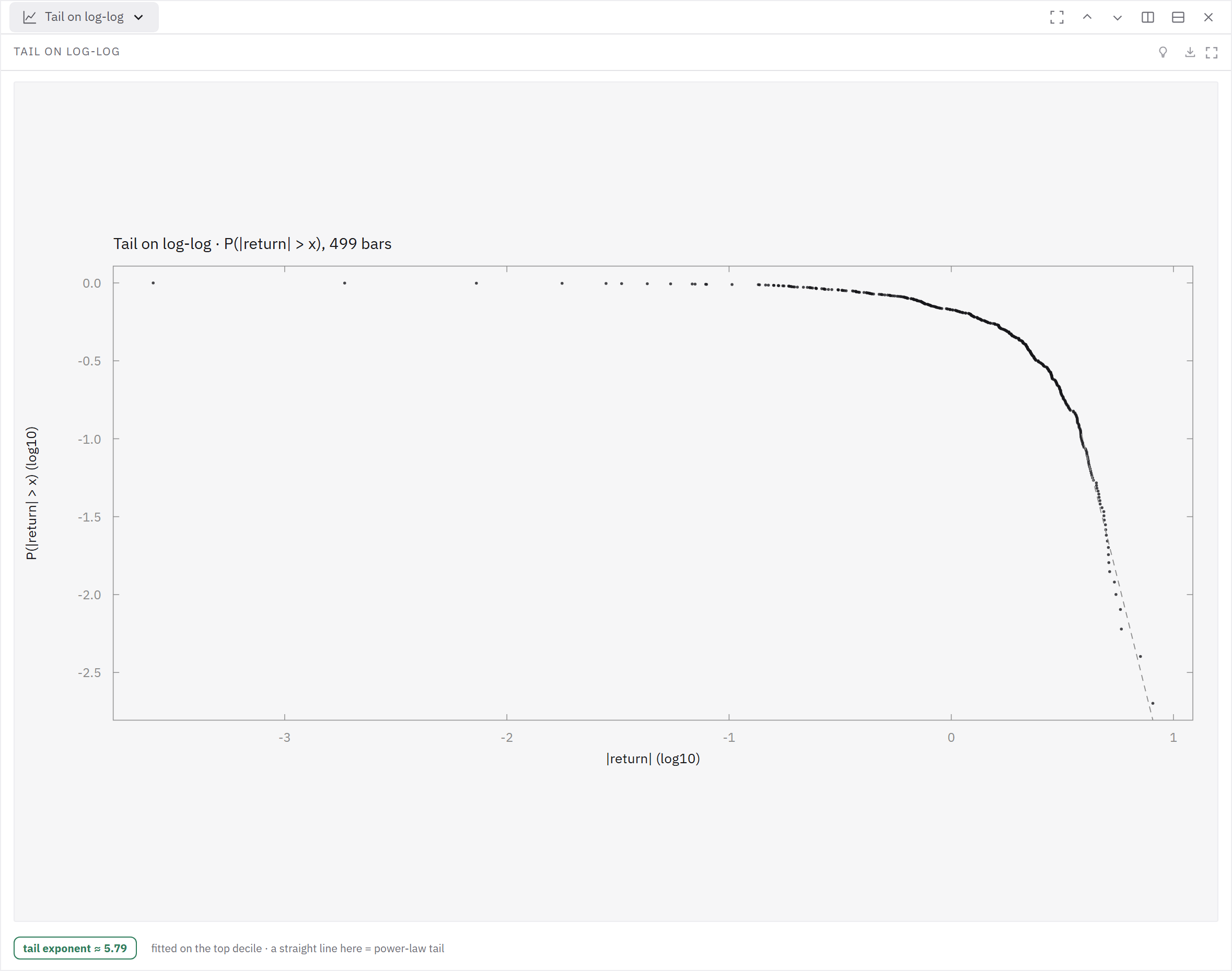
Gopikrishnan and coauthors found an approximate tail exponent near three over specified equity-index samples and horizons. Estimate your own tail threshold and uncertainty before using that model; another asset or longer horizon may have a different tail shape.
The observed tail exponent near three is bounded to the authors? equity-index samples and horizons.
Evidence map
| Aspect | Finding |
|---|---|
| What it is | The empirical finding that the tail of the distribution of returns, normalised by volatility, decays as a power law P(|r| > x) ~ x^(−α) with α close to 3. |
| Key result / formula | Gopikrishnan, Plerou, Amaral, Meyer & Stanley (1999) measured it on the S&P 500 with three databases — about one million one-minute records for 1984-1996, daily records for 1962-1996 and monthly records for 1926-1996. |
| Why it matters for backtesting | The measured tail exponent near three is a warning against fitting a Gaussian risk model without checking its tails. |
What it is
That is outside the Lévy-stable range α < 2, which the same measurement rules out: variance is finite, while the fourth moment sits at the edge of existence.
Key result / formula
The exponent α ≈ 3 holds for both tails from one minute up to horizons of a few days; at longer horizons the distribution slowly crosses over to a Gaussian. Gabaix, Gopikrishnan, Plerou & Stanley (2003) proposed a mechanism: large institutions whose sizes follow Zipf's law trade in markets where price impact is concave (square-root in volume), which turns the exponent 1 of fund sizes into an exponent 3 for returns and 3/2 for volumes — a derivation that predicts the two exponents jointly from one mechanism.
Why it matters for backtesting
The reported range belongs to the authors' equity-index samples and horizons; it is not a universal null for every market or period. At a specified confidence level, compare a Gaussian tail estimate with an empirical or suitably fitted heavy-tail estimate on the same data, then check exceedances out of sample. Whether the Gaussian estimate understates risk depends on the fitted distribution, horizon and quantile. A bootstrap or simulated null should preserve relevant dependence and tail behavior, but forcing an x^-3 law on a different asset could be just as misleading. Tail fitting also requires an explicit threshold and uncertainty interval; an eyeballed log-log slope does not establish an exponent. These constraints matter especially when the few most extreme observations dominate a risk estimate.
Source
Gopikrishnan, Plerou, Amaral, Meyer & Stanley, "Scaling of the distribution of fluctuations of financial market indices", Physical Review E 60(5), 1999, 5305-5316; Gabaix, Gopikrishnan, Plerou & Stanley, "A theory of power-law distributions in financial market fluctuations", Nature 423, 2003, 267-270. Primary source